The overview process of patient-specific heart modeling is: extract patient data to tune heart model parameters, next, initiate arrhythmia (the heart's initial state is also extracted from patient data), then solve the heart model equations to simulate patient-specific arrhythmias.
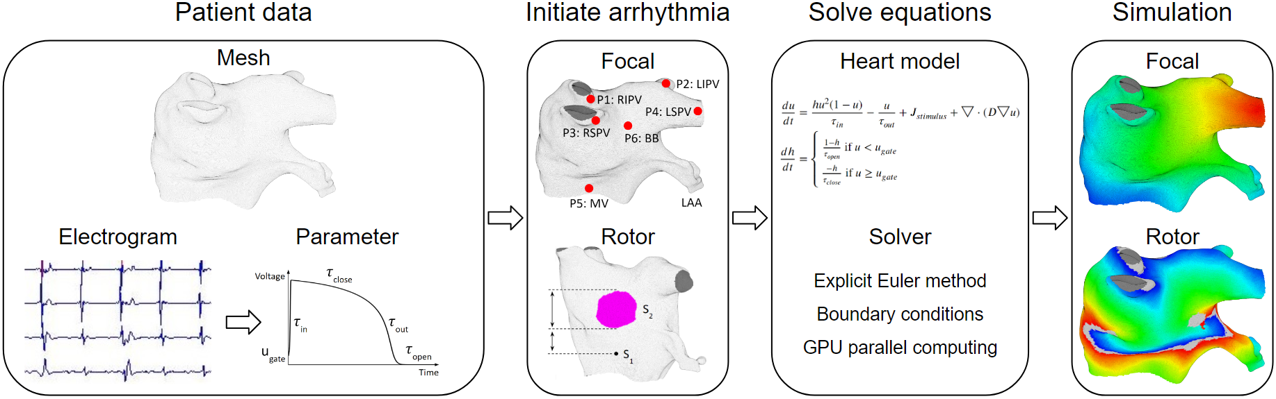
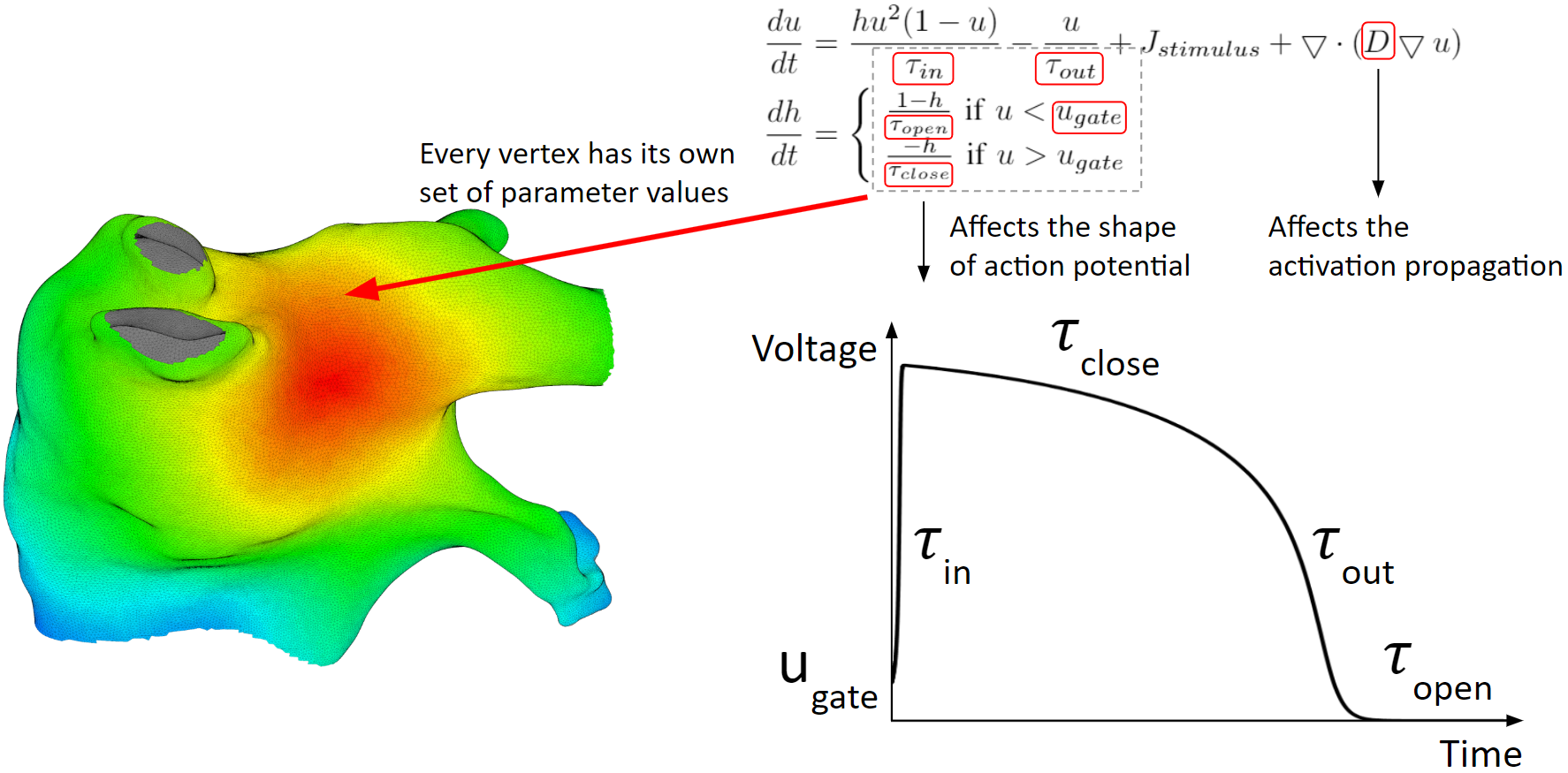
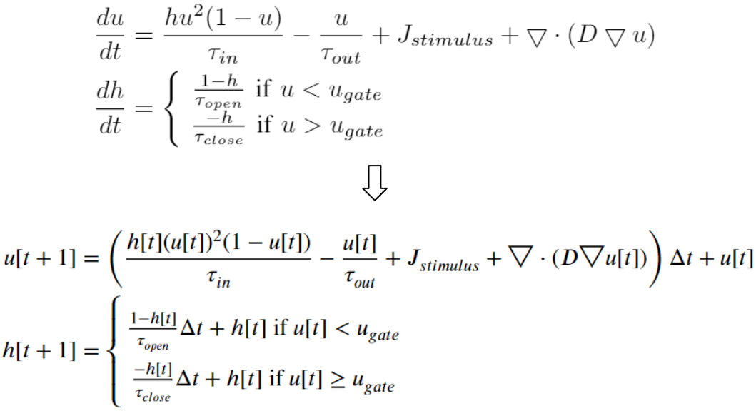
Below are the heart model equations. They calculate the activation action potentials. There are parameters that affect the shape of the action potential, and parameters that affect the activation propagation. These parameters are tuned locally. Every vertex of the mesh has its own set of parameter values.
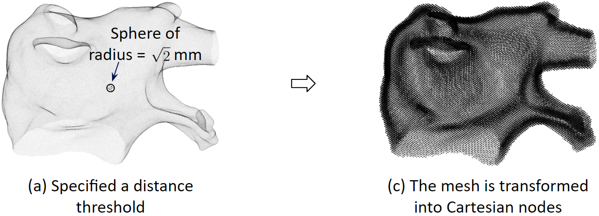
To solve the heart model equations, we discretize the left atrium in space. We transform the 3D triangular mesh into Cartesian nodes. For a mesh vertex, Cartesian nodes within a radius are created. And for every vertex, we create the associated cartesian nodes. As a result, the Cartesian nodes will wrap around the mesh.
We discretize the heart model equations in time using the explicit Euler method. With some initial values at time 0, we can compute the values of the next time step.
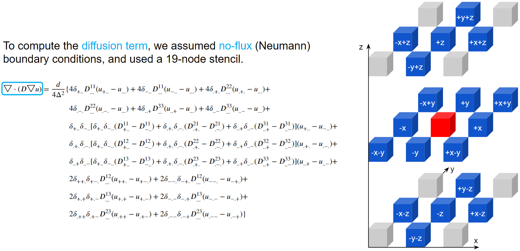
To compute the diffusion term, we assumed no-flux boundary conditions, and used a 19-node stencil. The action potential of the red node will be diffused into its 18 neighbors according to the diffusion coefficient matrices.
Here are examples of arrhythmia simulations. Focal arrhythmia: Activation originates at an abnormal location. Rotor arrhythmia: Spiral waves cause irregular heartbeat. Zigzag propagation: Complex scar distributions create activation tunnels of various conduction velocities. Atrial fibrillation: Chaotic activation waves that have no organizations.
Our solution to the lack of fiber data is to compensate that with a diffusion coefficient tuning. Tuning is challenging: 1) Heart model is nonlinear. 2) Diffusion is influencing the neighbor nodes, not the immediate vicinities. 3) Sensitive to the initial guess values, adjustment steps, ending criteria, etc.
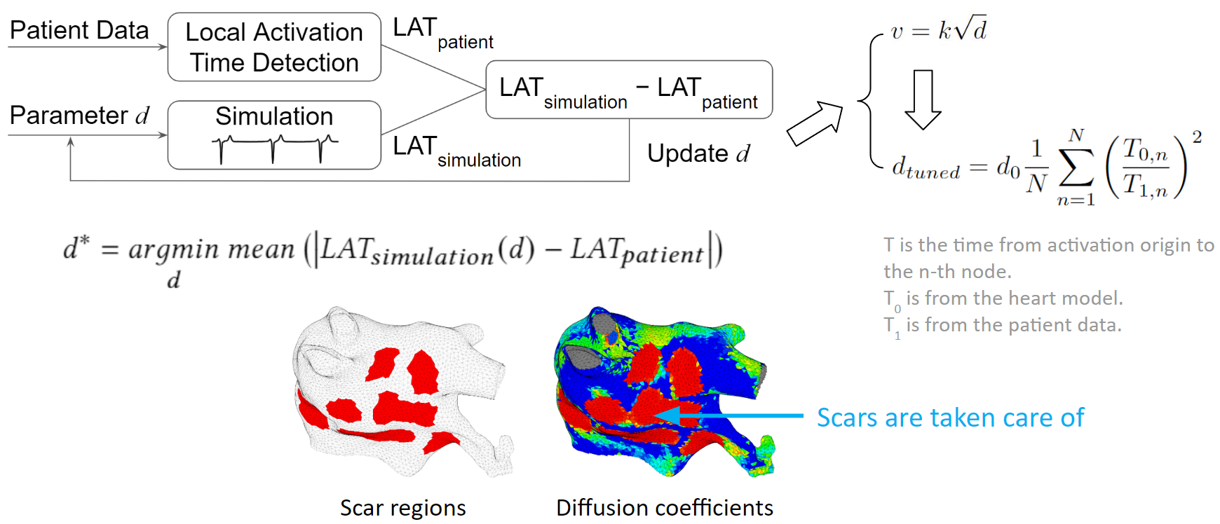
We developed an optimization process to overcome the tuning challenges. We process the patient data to obtain the true local activation times. Then we run a simulation with some initial guess diffusions, and process the simulation result to obtain the simulated local activation times. These two sets of activation times are compared and the diffusion values are updated according to this comparison. New simulations are run and diffusion values are adjusted in each iteration. The tuning is done when the difference between patient activation time and simulation activation time is minimized. To make the tuning faster, we exploit the relation between conduction velocity and diffusion coefficient, which reduces the number of iterations needed to reach the optimum. As illustrated in the figure below, we can see that scars are taken care of too. The figure on the left shows scar regions in red, and the figure on the right, shows a diffusion coefficient map, where red represents low conductivity. The red regions between these two figures are almost the same. Which means the tuning is accurate.
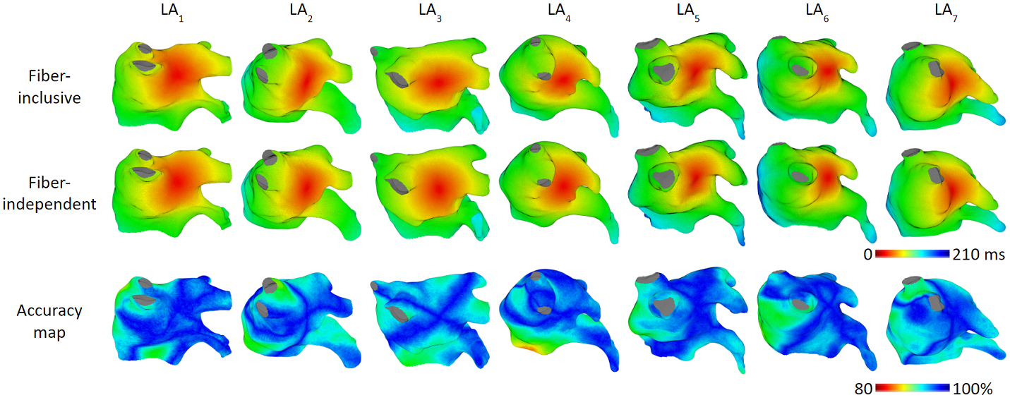
Our model achieved high accuracy of simulating arrhythmias. We ran experiments on 7 patient’s left atrium. For focal arrhythmia, we achieved activation time accuracy of 96%.
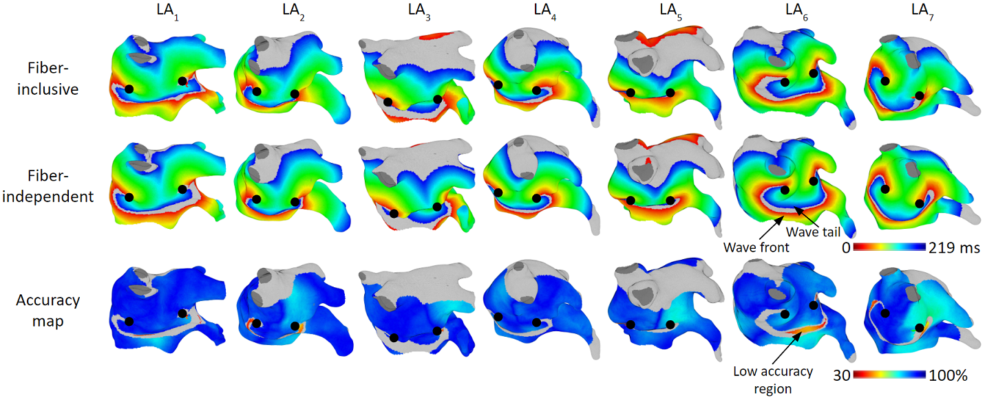
For rotor arrhythmia, we achieved activation time accuracy of 93%.
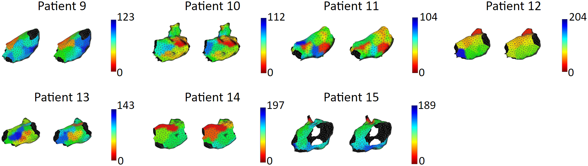
We tested our model with 15 patient data, to show that our model is capable of accurately reproducing patient arrhythmias. The figures below are the results of 7 atrial tachycardia maps. We achieved an average activation time error of 10.97 ms, with an average correlation of 0.81.
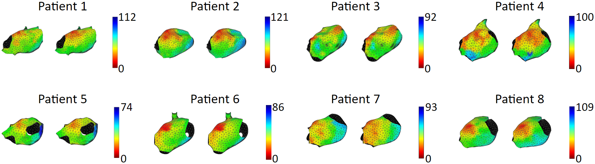
These are the results of 8 sinus rhythm maps. We achieved an average activation time error of 5.47 ms, with an average correlation of 0.95. Sinus rhythm maps are helpful: Oftentimes, patient comes in the operating room in sinus rhythm, or will get cardioversion into sinus rhythm, to acquire a voltage map for assisting pulmonary vein isolation.